Mathematical Trading: Your Complete Guide to the Mathematics of Stock Market Success

Have you ever wondered how Wall Street quants and successful traders seem to predict market moves with uncanny accuracy? The secret isn’t a crystal ball—it’s mathematics. In this comprehensive guide, we’ll demystify mathematical trading, breaking down complex concepts into bite-sized, actionable insights that will give you a significant edge in today’s competitive markets.

What is Mathematical Trading and Why Should You Care?

Mathematical trading (also known as quantitative trading) utilizes mathematical models, statistical analysis, and computational algorithms to identify and execute trading opportunities in financial markets. Unlike regular trading that depends a lot on gut feeling and basic company analysis, mathematical trading uses precision methods, making decisions more accurate, consistent, and easy to scale.

Essential Mathematical Concepts Every Trader Should Master

1. Statistical Analysis: The Foundation of Market Understanding

At the core of mathematical trading lies statistical analysis, helping traders make sense of market data and identify profitable opportunities.

Measures of Central Tendency

Mean (Average)

The mean represents the average value in a dataset and is calculated as:

Mean = (x₁ + x₂ + x₃ + ... + xₙ) / n

In trading, means are frequently used in moving averages—powerful technical indicators that smooth price data to identify trends.

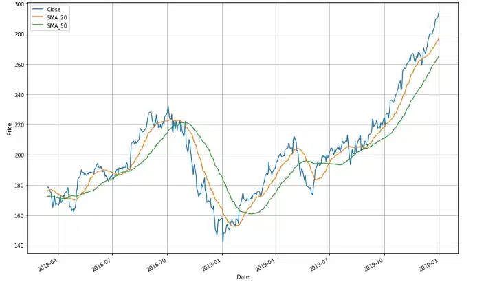
Trading Application: When a shorter-period moving average (like 20 days) crosses above a longer-period moving average (like 50 days), it generates a bullish signal, suggesting it might be time to buy. Conversely, when the shorter-period moving average crosses below the longer one, it indicates a bearish signal—potentially time to sell.

Median and Mode

While the mean can be skewed by outliers, the median (middle value when data is ordered) provides a more robust measure of central tendency, especially in volatile markets.

# Python code for calculating median of stock prices
import numpy as np
import yfinance as yf

# Download historical data for Apple
aapl = yf.download('AAPL', start='2024-01-01', end='2024-05-14')
median_price = np.median(aapl['Close'])
print(f"Median Apple stock price: ${median_price:.2f}")

Measures of Dispersion

Standard Deviation

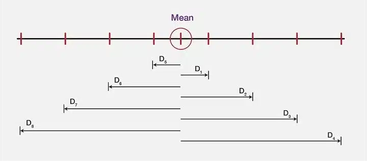
Standard deviation measures the amount of variation or dispersion in a dataset, calculated as:

σ = √[(Σ(x - μ)²) / N]

Where σ is the standard deviation, x represents each value in the dataset, μ is the mean, and N is the total number of values.

Trading Application: Standard deviation is the foundation of volatility measurement in finance. Higher standard deviation indicates greater price volatility and potentially higher risk. It’s essential for:

• Setting stop-loss levels
• Options pricing models
• Risk assessment in portfolio construction
• Volatility-based trading strategies like Bollinger Bands

2. Probability Theory: Dealing with Uncertainty

Markets are inherently unpredictable, but probability theory helps traders quantify and manage uncertainty.

Random Walk and Efficient Market Hypothesis

The Random Walk Theory says that stock prices change in a random way, so it’s not possible to reliably guess future prices just by looking at past trends. This theory aligns with the Efficient Market Hypothesis, which posits that asset prices reflect all available information.

Trading Application: Understanding random walk helps traders:

• Avoid overreacting to short-term price movements
• Focus on statistical edges rather than perfect predictions
• Develop strategies that account for market randomness

Monte Carlo Simulation

Monte Carlo simulation is a powerful technique that uses random sampling to model the probability of different outcomes in a process that cannot be easily predicted due to random variables.

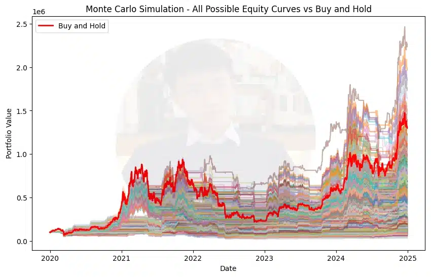
Trading Application: Monte Carlo simulations help traders:

3. Calculus: Understanding Rate of Change

Calculus is essential for modeling continuous change in financial markets. The two main branches relevant to trading are:

1. Differential Calculus: Calculates instantaneous rates of change (derivatives)
2. Integral Calculus: Calculates accumulated values over time (integrals)

Trading Application: Calculus is fundamental to:

• Option pricing models like Black-Scholes
• Risk measures like Delta, Gamma, and Theta in options trading
• Understanding price momentum and acceleration
• Building continuous-time financial models

4. Linear Algebra: Multi-dimensional Analysis

Linear algebra provides tools for managing and analyzing multi-dimensional data, making it indispensable for modern quantitative finance.

Matrices and Vectors

Matrices allow traders to work with large datasets efficiently. A portfolio of assets can be represented as a vector, with each element corresponding to the weight of a particular asset.

Trading Application:

• Portfolio optimization (Modern Portfolio Theory)
• Factor models for returns (like Fama-French models)
• Correlation analysis between multiple assets
• Dimension reduction techniques like Principal Component Analysis (PCA)

5. Regression Analysis: Finding Relationships

Regression analysis identifies relationships between variables, helping traders understand how different factors influence asset prices.

Linear Regression

The basic formula for linear regression is:

Y = mX + b

Where Y is the dependent variable (e.g., stock price), X is the independent variable (e.g., market index), m is the slope, and b is the y-intercept.

Trading Applications:

• Identifying relationships between assets (pairs trading)
• Measuring a stock’s sensitivity to the market (beta)
• Trend analysis and price prediction
• Mean reversion strategies

Advanced Mathematical Frameworks for Trading Success

1. Modern Portfolio Theory (MPT)

Developed by Harry Markowitz in the 1950s, MPT provides a mathematical framework for assembling a portfolio of assets that maximizes expected return for a given level of risk.

Key Concepts:

• Efficient Frontier: The set of optimal portfolios that offer the highest expected return for a defined level of risk
• Diversification: The mathematical proof that proper asset allocation can reduce portfolio risk
• Capital Allocation Line: The line representing all possible combinations of the risk-free asset and the risky portfolio

# Simplified Modern Portfolio Theory example
import numpy as np
import pandas as pd
import yfinance as yf
import matplotlib.pyplot as plt
from scipy.optimize import minimize

# Download data for two stocks
tickers = ['AAPL', 'MSFT']
start_date = '2023-05-14'
end_date = '2024-05-14'

data = yf.download(tickers, start=start_date, end=end_date)['Adj Close']
returns = data.pct_change().dropna()

# Calculate mean returns and covariance matrix
mean_returns = returns.mean()
cov_matrix = returns.cov()

# Function to calculate portfolio performance
def portfolio_performance(weights, mean_returns, cov_matrix):
    returns = np.sum(mean_returns * weights) * 252
    std = np.sqrt(np.dot(weights.T, np.dot(cov_matrix, weights))) * np.sqrt(252)
    return std, returns

# Function to minimize for finding minimum volatility portfolio
def min_variance(weights, mean_returns, cov_matrix):
    return portfolio_performance(weights, mean_returns, cov_matrix)[0]

# Constraints and bounds
constraints = {'type': 'eq', 'fun': lambda x: np.sum(x) - 1}
bounds = tuple((0, 1) for asset in range(len(tickers)))
initial_guess = [1/len(tickers)] * len(tickers)

# Optimize for minimum volatility
min_vol_result = minimize(min_variance, initial_guess, 
                          args=(mean_returns, cov_matrix),
                          method='SLSQP', bounds=bounds, constraints=constraints)

min_vol_weights = min_vol_result['x']
min_vol_std, min_vol_ret = portfolio_performance(min_vol_weights, mean_returns, cov_matrix)

print(f"Minimum Volatility Portfolio:")
print(f"Annual Return: {min_vol_ret:.4f}")
print(f"Annual Volatility: {min_vol_std:.4f}")
print("Asset Allocation:")
for i, ticker in enumerate(tickers):
    print(f"{ticker}: {min_vol_weights[i]:.4f}")

2. Factor Models

Factor models decompose asset returns into systematic components (factors) and idiosyncratic components. The most famous is the Capital Asset Pricing Model (CAPM), expressed as:

E(Ri) = Rf + βi(E(Rm) - Rf)

Where:

• E(Ri) is the expected return of the asset
• Rf is the risk-free rate
• βi is the beta of the asset
• E(Rm) is the expected return of the market

Trading Applications:

• Risk factor decomposition
• Alpha generation (returns unexplained by common factors)
• Risk-adjusted performance evaluation
• Smart beta strategies

3. Stochastic Processes

Stochastic processes model random changes over time, which is perfect for financial markets. These models include:

1. Brownian Motion: Models random price movements
2. Geometric Brownian Motion: Models percentage price changes
3. Mean-Reverting Processes: Models prices that tend to revert to a mean
4. Jump-Diffusion Models: Incorporates sudden price jumps

Trading Applications:

• Option pricing models
• Volatility modeling
• Risk management
• High-frequency trading algorithms

Market-Beating Mathematical Trading Strategies

Let’s explore some practical trading strategies that leverage mathematical concepts:

1. Mean Reversion Strategy

Mean reversion strategies capitalize on the tendency of asset prices to return to their historical average over time.

Mathematical Foundation:

• Standard deviation to identify overbought/oversold conditions
• Z-scores to quantify deviations from the mean
• Statistical tests for stationarity (e.g., Augmented Dickey-Fuller test)

Trading Algorithm:

1. Calculate the historical mean and standard deviation of a price series
2. Enter a long position when the price falls below μ – 2σ (two standard deviations below the mean)
3. Enter a short position when the price rises above μ + 2σ (two standard deviations above the mean)
4. Exit when the price reverts to the mean

2. Momentum Strategy

Momentum strategies leverage the tendency of assets that have performed well (or poorly) in the recent past to continue their performance in the near future.

Mathematical Foundation:

• Rate of change calculations
• Regression analysis for trend identification
• Statistical significance testing

Trading Algorithm:

1. Calculate the n-period return for all assets in the universe
2. Rank assets based on their returns
3. Go long the top-performing decile and short the bottom-performing decile
4. Rebalance at regular intervals (e.g., monthly)

3. Statistical Arbitrage

Statistical arbitrage exploits price inefficiencies between related assets using mathematical models.

Mathematical Foundation:

• Cointegration analysis
• Regression for estimating spread relationships
• Statistical tests for mean reversion

Trading Algorithm:

1. Identify pairs of cointegrated assets
2. Calculate the spread between the assets
3. Standardize the spread to identify extreme values
4. Go long the undervalued asset and short the overvalued asset when the spread exceeds a threshold
5. Unwind the position when the spread reverts to the mean

4. Machine Learning-Enhanced Strategies

Advanced mathematical techniques like machine learning can significantly enhance trading strategies by identifying complex patterns in market data.

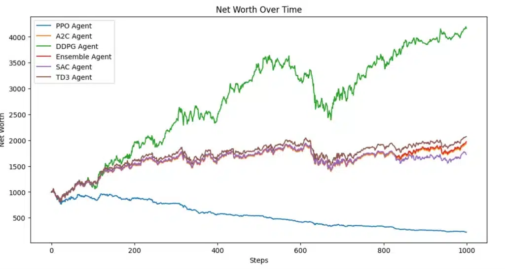
Mathematical Foundation:

• Supervised learning algorithms (e.g., random forests, neural networks)
• Feature engineering and selection
• Cross-validation and overfitting prevention
• Performance metrics (e.g., Sharpe ratio, drawdown)

Risk Management Mathematics: Protecting Your Capital

Even the best mathematical trading strategies can fail without proper risk management. Here’s how mathematics helps traders protect their capital:

1. Value at Risk (VaR)

VaR estimates the maximum potential loss a portfolio might experience over a specific time period at a given confidence level.

Formula:

VaR = μ + σ × z

Where μ is the portfolio’s expected return, σ is the portfolio’s standard deviation, and z is the z-score corresponding to the desired confidence level (e.g., -1.645 for 95% confidence).

Trading Application: VaR helps traders:

• Set position sizes
• Allocate risk capital
• Report potential losses to stakeholders
• Comply with regulatory requirements

2. Position Sizing Models

Mathematics provides rigorous frameworks for determining optimal position sizes, such as the Kelly Criterion:

f* = (p × b - q) / b

Where f* is the optimal fraction of capital to risk, p is the probability of winning, q is the probability of losing (1-p), and b is the odds received on the wager.

Trading Application: Proper position sizing helps traders:

• Maximize long-term growth rate
• Avoid risk of ruin
• Balance risk and reward
• Manage drawdowns

3. Correlation Analysis

Correlation measures the strength and direction of the linear relationship between two variables, ranging from -1 (perfect negative correlation) to +1 (perfect positive correlation).

Trading Application: Correlation analysis helps traders:

• Build truly diversified portfolios
• Identify pairs trading opportunities
• Hedge portfolio risks
• Detect changes in market regimes

Practical Implementation: Building Your First Mathematical Trading System

Now that we’ve covered the theoretical foundations, let’s put it all together with a step-by-step guide to building your first mathematical trading system.

Step 1: Define Your Strategy Objectives

• Time horizon (intraday, swing, long-term)
• Expected return and risk tolerance
• Markets and instruments
• Capital requirements

Step 2: Collect and Preprocess Data

• Historical price and volume data
• Fundamental data (if applicable)
• Alternative data sources
• Data cleaning and normalization

Step 3: Develop Your Mathematical Model

• Select appropriate mathematical techniques
• Engineer features based on domain knowledge
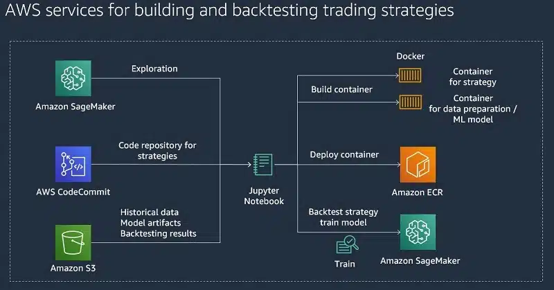
• Implement backtesting framework
• Optimize parameters (but avoid overfitting)

Step 4: Implement Risk Management Rules

• Position sizing rules
• Stop-loss and take-profit levels
• Portfolio-level risk constraints
• Drawdown management

Step 5: Evaluate Performance

• Calculate key performance metrics
• Test robustness across different market regimes
• Perform out-of-sample testing
• Consider transaction costs and slippage

Step 6: Deploy and Monitor

• Set up execution infrastructure
• Implement real-time monitoring
• Establish performance tracking
• Plan for periodic strategy review

Market Overview: What’s Driving Mathematical Trading in 2025?

The landscape of mathematical trading continues to evolve rapidly. Here are the key developments shaping the field in 2025:

1. AI and Deep Learning Revolution

Machine learning models, particularly deep neural networks, are revolutionizing quantitative trading by:

• Identifying complex, non-linear patterns in market data
• Processing unstructured data like news and social media
• Adapting to changing market conditions through reinforcement learning
• Optimizing execution algorithms for minimal market impact

2. Alternative Data Integration

Mathematical traders are gaining edges by incorporating alternative data sources:

• Satellite imagery for supply chain analysis
• Credit card transaction data for consumer spending insights
• Mobile location data for retail foot traffic
• Natural language processing of earnings calls and financial news

3. Quantum Computing on the Horizon

While still in its early stages, quantum computing promises to transform mathematical trading by:

• Solving complex optimization problems instantaneously
• Simulating financial markets with unprecedented accuracy
• Accelerating risk calculations and option pricing
• Breaking current encryption methods for secure financial transactions

Behavioral Finance: The Human Element

Even with sophisticated mathematical models, markets are ultimately driven by human behavior. Modern mathematical trading incorporates behavioral finance insights by:

1. Quantifying Sentiment: Using natural language processing to measure market sentiment from news, social media, and analyst reports
2. Modeling Behavioral Biases: Incorporating well-documented biases like loss aversion, herding, and overconfidence into trading models
3. Regime Detection: Identifying when markets shift between rational and emotional states to adapt strategy parameters accordingly
4. Contrarian Indicators: Using extreme sentiment readings as contrarian signals for mean reversion strategies

Building Your Mathematical Trading Toolkit

To implement the strategies discussed in this article, you’ll need the right tools and resources:

Essential Software and Libraries

1. Programming Languages:
   • Python (pandas, numpy, scikit-learn, TensorFlow, PyTorch)
   • R (quantmod, xts, PerformanceAnalytics)
   • Julia (for high-performance computing)
2. Backtesting Platforms:
   • Backtrader
   • QuantConnect
   • Zipline
   • Amibroker
3. Data Providers:
   • Alpha Vantage
   • Quandl
   • Bloomberg
   • Refinitiv

Learning Resources

1. Books:
   • “Advances in Financial Machine Learning” by Marcos Lopez de Prado
   • “Statistical Arbitrage” by Andrew Pole
   • “Options, Futures, and Other Derivatives” by John Hull
2. Online Courses:
   • Financial Engineering and Risk Management (Columbia University)
   • Algorithmic Trading and Finance Models with Python, R, and Stata (New York University)
   • Machine Learning for Trading (Georgia Tech)
3. Research Papers:
   • Journal of Portfolio Management
   • Journal of Financial Markets
   • Journal of Investment Strategies

Conclusion: The Future of Mathematical Trading

The mathematics of stock markets has evolved from simple formulas to sophisticated algorithms powered by artificial intelligence. While mastering these concepts requires dedication, the potential rewards—both in terms of financial returns and intellectual satisfaction—are substantial.

As we look to the future, mathematical trading will continue to become more accessible to individual traders while simultaneously pushing the boundaries of innovation at institutional levels. Success will come to those who can effectively combine mathematical rigor with adaptability and risk management discipline.

Remember that no mathematical model is perfect, and markets will always find ways to surprise even the most sophisticated traders. The key is to use mathematics as a powerful tool in your trading arsenal while maintaining humility about the inherent uncertainties of financial markets.

Actionable Steps to Get Started

1. Master the foundational mathematical concepts covered in this guide
2. Start with simple models and gradually increase complexity
3. Build a robust backtesting framework to validate your strategies
4. Implement proper risk management from day one
5. Join communities of like-minded quantitative traders for continuous learning

Frequently Asked Questions

Q: Do I need an advanced mathematics degree to use mathematical trading strategies?

A: No. While a strong foundation in mathematics is helpful, many successful traders have learned the necessary concepts through self-study and practical application. Start with basic concepts like mean, standard deviation, and correlation, then gradually progress to more advanced topics.

Q: Are mathematical trading strategies guaranteed to be profitable?

A: Absolutely not. Even the most sophisticated mathematical models have limitations and can fail during extreme market conditions or regime changes. That’s why proper risk management is essential to long-term success.

Q: How much capital do I need to start with mathematical trading?

A: It depends on your strategy. Some high-frequency strategies require substantial capital and sophisticated infrastructure, while many statistical arbitrage and momentum strategies can be implemented with more modest capital. Focus first on developing and validating your strategy before scaling up with real capital.

Q: How can I avoid overfitting my mathematical models?

A: Use out-of-sample testing, cross-validation, and walk-forward optimization. Keep your models as simple as possible while still capturing the essential patterns. Be skeptical of strategies that perform exceptionally well in backtests but have no economic rationale.

Q: Can mathematical trading strategies still work if everyone is using them?

A: When strategies become overcrowded, their effectiveness can diminish—a phenomenon known as alpha decay. However, markets are continuously evolving, creating new inefficiencies and opportunities for those who can adapt their models accordingly.

Q: Which programming language is best for mathematical trading?

A: Python has emerged as the dominant language due to its extensive libraries for data analysis and machine learning. However, R excels at statistical analysis, and C++ offers superior performance for high-frequency strategies. Choose the language that best fits your specific needs and existing skills.

Q: How do I stay updated with the latest developments in mathematical trading?

A: Follow academic journals like the Journal of Portfolio Management, attend conferences such as QuantCon, join online communities like QuantConnect, and continuously experiment with new techniques and data sources.

Suggested Internal Links:

1. “Beginner’s Guide to Technical Analysis“
2. “Understanding Market Volatility“

Suggested External Links:

1. Federal Reserve Economic Data (FRED)
2. MIT OpenCourseWare: Mathematics for Computer Science
3. CFA Institute Research Foundation

Suggested Videos: